Taylor Expansion – Chan’s Research Note

Package Import

import numpy as np
import scipy
import matplotlib.pyplot as plt

Note

This content is a summary of Börge Göbel’s “Computational Physics: Scientific Programming with Python” on Udemy.

Why Taylor Expansion?

The reason for using Taylor Expansion is to approximate complex functions into simple polynomial forms. When studying mathematics, various formulas appear, and the original forms of the equations we often encounter in theory are usually composed of trigonometric or exponential functions. Operations between these functions are too complex and computationally expensive to calculate directly, but using Taylor Expansion, these complex expressions can be easily represented. For example, if the derivative of a function can be calculated, an approximate value of the function for a specific point can be expressed using this derivative.

\[f(x)=\sum_{n=0}^\infty \frac{1}{n!}f^{(n)}(x_0)\,(x-x_0)^n\]

Here, \(f^{(n)}\) is the \(n\)-th derivative of \(f(x)\), and \(x_0\) represents the position of the value we want to calculate.

1.1 Exponential Function

If the original form of the function we want to find is an exponential function, we can easily apply the Taylor Expansion.

\[f(x)=f'(x)=f''(x)=\dots=f^{(n)}(x)=\exp(x)\]

This is because the derivative of the exponential function is the exponential function itself. The code and visualization for this can be expressed as follows.

def ExpTaylor(x, x0, nmax):
    t = 0
    for n in range(nmax + 1):
        t = t + (np.exp(x0) * (x - x0) ** n) / scipy.special.factorial(n)
    return t

Note

In the original example, np.math.factorial was used for the factorial calculation, but the math sub-package was not originally provided by numpy. So, as the version was updated and math was removed, the example above was changed to calculate it through scipy.special. The result is the same as we think.

np.exp(1), ExpTaylor(1, 0, 10)

(np.float64(2.718281828459045), np.float64(2.7182818011463845))

So, if you compare the actual value of the natural function with the approximate value, you can see that they are quite similar.

x_list = np.linspace(-5, 5, 101)
plt.ylim([-5, 100])

plt.xlabel('x')
plt.ylabel('y')
plt.scatter(x_list, np.exp(x_list), label='exponential')

nmax = 5
plt.plot(x_list, ExpTaylor(x_list, 0, nmax), c='blue', label='$x_0$=0')
plt.plot(x_list, ExpTaylor(x_list, -3, nmax), c='red', label='$x_0$=-3')
plt.plot(x_list, ExpTaylor(x_list, 2, nmax), c='green', label='$x_0$=2')
plt.legend()
plt.show()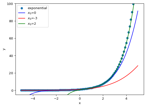

In fact, it is an area of approximation to reduce the amount of computation, and the part that cannot accurately represent the function can be seen just by checking the result of changing the initial point. However, if an appropriate initial point is selected, an approximate value that is close to the original function we want to find can be obtained.

1.2 Sin function at \(x_0=0\)

The Taylor expansion of the sin function among trigonometric functions is expressed as follows.

\(f(0) = f''(0) = f^{(4)}(0) = \dots = 0\)

\(f'(0) = f^{(5)}(0) = f^{(9)}(0) = \dots = 1\)

\(f'''(0) = f^{(7)}(0) = f^{(11)}(0) = \dots = -1\)

\(\sin(x) = x - \frac{1}{3!}x^3 + \frac{1}{5!}x^5 - \frac{1}{7!}x^7 \pm \dots = \sum_{n=0}^\infty \frac{(-1)^n}{(2n+1)!}x^{2n+1}\)

def SinTaylor(x, nmax):
    t = 0
    for n in range(nmax + 1):
        t = t + ((-1) ** n / scipy.special.factorial(2 * n + 1)) * (x ** (2 * n + 1))
    return t

x_list = np.linspace(-10, 10, 101)
plt.ylim([-2, 2])

plt.xlabel('x')
plt.ylabel('y')
plt.scatter(x_list, np.sin(x_list), label='sine')

plt.plot(x_list, SinTaylor(x_list, 3), c='blue', label='$x_0$=0')
plt.plot(x_list, SinTaylor(x_list, 6), c='red', label='$x_0$=-3')
plt.plot(x_list, SinTaylor(x_list, 10), c='green', label='$x_0$=10')
plt.plot(x_list, SinTaylor(x_list, 20), c='black', label='$x_0$=20')
plt.legend()
plt.show()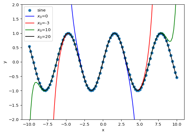

np.sin(2.5), SinTaylor(2.5, 10)

(np.float64(0.5984721441039565), np.float64(0.598472144104011))

1.3 Implementation of General Function

The previous example was shown assuming that the derivative for a simple function is known, and the formula for obtaining the actual derivative is as follows.

\[f'(x) = \lim_{h\rightarrow 0} \frac{f(x+h)-f(x)}{h}\]

def derivative(f, x, h):
    # Adding Small number to avoid ZeroDivision Error
    return (f(x + h) - f(x)) / (h + 0.000001)

However, the above formula was for obtaining the first derivative, and the \(n\)-th derivative, which is differentiated \(n\) times, is obtained by repeatedly performing the above formula, which is expressed a little more complicatedly as follows.

\[f^{(n)}(x) = \lim_{h\rightarrow 0} \frac{1}{h^n}\sum_{k=0}^n(-1)^{k+n} \,\frac{n!}{k!(n-k)!} \,f(x+kh)\]

def nDerivative(f, x, h, n):
    t = 0
    for k in range(n + 1):
        t = t + (-1) **(k + n) * scipy.special.factorial(n) / (scipy.special.factorial(k) * scipy.special.factorial(n - k)) * f(x + k * h)
    return t / (h ** n)

let’s find the derivative for the following equation.

\[f(x) = 2 * \sin^2(x) + x\]

def func(x):
    return 2 * np.sin(x) ** 2 + x

x0 = 10.5
h = 0.1

func(x0)

np.float64(12.04772926022427)

derivative(func, x0, h)

np.float64(2.5529714426967454)

nDerivative(func, x0, h, 0), nDerivative(func, x0, h, 1), nDerivative(func, x0, h, 2)

(np.float64(12.04772926022427),
 np.float64(2.5529969724111723),
 np.float64(-2.802754599797907))

nDerivative(func, x0, h, 1)

np.float64(2.5529969724111723)

1.4 Taylor Expansion of General Function

Now, let’s bring back the Taylor Expansion formula introduced at the beginning:

\[f(x)=\sum_{n=0}^\infty \frac{1}{n!}f^{(n)}(x_0)\,(x-x_0)^n\]

Ultimately, this formula allows for approximation only if the derivative of the function can be found. Now, let’s replace the derivative part with the function defined above.

def taylor(f, x, x0, nmax, h):
    t = 0
    for n in range(nmax + 1):
        t = t + nDerivative(f, x0, h, n) * (x - x0) ** n / scipy.special.factorial(n)
    return t

First, if we approximate with 5 samples and set the derivative step to 0.1, it approximates well within a certain range, but if it goes out of range, the value jumps out.

x_list = np.linspace(-5, 5, 101)
plt.ylim([-10, 10])

plt.xlabel('x')
plt.ylabel('y')
plt.scatter(x_list, func(x_list), label='sin')

nmax = 5
h = 0.1

plt.plot(x_list, taylor(func, x_list, 0, nmax, h), c='blue', label='$x_0$=0')
plt.plot(x_list, taylor(func, x_list, 2, nmax, h), c='red', label='$x_0$=2')
plt.plot(x_list, taylor(func, x_list, -3, nmax, h), c='green', label='$x_0$=-3')
plt.legend()
plt.show()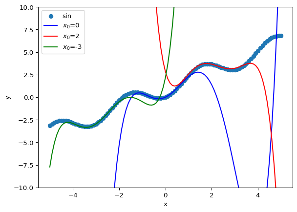

If nmax is increased by 10, the output gets more accurate result besides previous ones.

x_list = np.linspace(-5, 5, 101)
plt.ylim([-10, 10])

plt.xlabel('x')
plt.ylabel('y')
plt.scatter(x_list, func(x_list), label='sin')

nmax = 10
h = 0.1

plt.plot(x_list, taylor(func, x_list, 0, nmax, h), c='blue', label='$x_0$=0')
plt.plot(x_list, taylor(func, x_list, 2, nmax, h), c='red', label='$x_0$=2')
plt.plot(x_list, taylor(func, x_list, -3, nmax, h), c='green', label='$x_0$=-3')
plt.legend()
plt.show()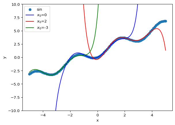

Additionally, we can get more accurate result if we decrease the step size that used to calculate the derivative.

x_list = np.linspace(-5, 5, 101)
plt.ylim([-10, 10])

plt.xlabel('x')
plt.ylabel('y')
plt.scatter(x_list, func(x_list), label='sin')

nmax = 10
h = 0.01

plt.plot(x_list, taylor(func, x_list, 0, nmax, h), c='blue', label='$x_0$=0')
plt.plot(x_list, taylor(func, x_list, 2, nmax, h), c='red', label='$x_0$=2')
plt.plot(x_list, taylor(func, x_list, -3, nmax, h), c='green', label='$x_0$=-3')
plt.legend()
plt.show()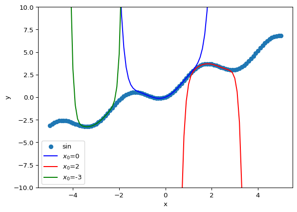

In short, if a function is computationally expensive to evaluate, obtaining its derivative can help. Additionally, the more samples you have of the function, the better you can approximate its true value.

Reuse

CC BY 4.0